Stable Diffusion

Introduction
Stable Diffusion is an AI text to image generator made using Deep Learning. Diffusion models gained popularity due to less time and data required to train, beating the likes of GAN. In this blog we will understand how stable diffusion technology works in detail.
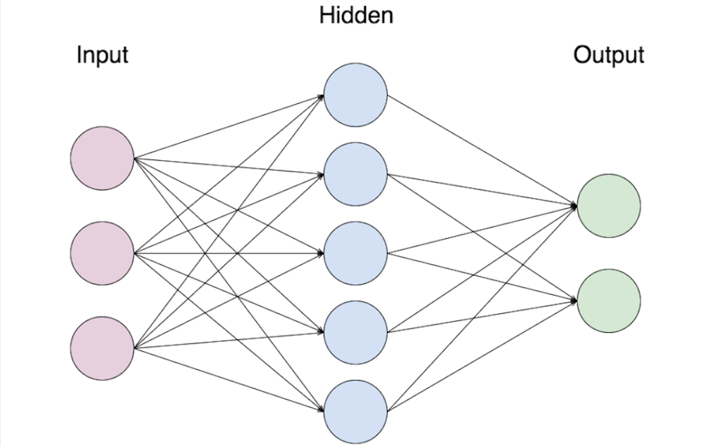
Deep learning is all about neural networks and how they are connected. There are many different ways neurons can be connected one of it being fully connected neural network, where every neuron in each layer is connected to every neuron in another layer, a very basic one. Ofcourse this cant be used in image generation, say you take 128x128 res image, that's 16384 parameters in input and you want to generate 128x128 image, another 16,384 parameters. If you want to connect both input and output by basic neural layers, it will be 16,384x16,384 connections. This is definitely a lot of data to consider for just a 128x128 image, hence networks like basic neural network fall off.
Diffusion model uses 2 layers:
- Convolusional Layer
- Attention Layer
What is Convolution ?
Say you take a dice, roll and make a table based on all possible results.
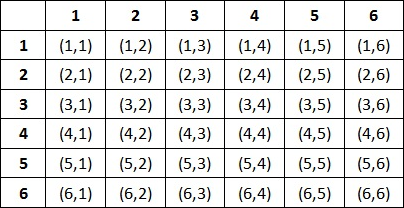
P(sum) = elements in the diagnol/total possiblities
Another way of representing this is by superimposing one dice possiblities and another dice possiblities (inverted). Like,
1 2 3 4 5 6
6 5 4 3 2 1
(Note that probablity of each pair is product of probablity of each element appearing in a pair => 1/6*1/6 = 1/36 in an unbiased dice. This notation will be used later.)
You will notice that elements in the same column give sum of 7. Six columns=> P(sum = 7) = 6/36.(6*1/36, sum of each pair's probablity = 1/36+1/36+1/36+1/36+1/36+1/36. This notation will be used later.) If you move the bottom dice once towards right,
1 2 3 4 5 6
6 5 4 3 2 1
you can notice that each column give sum of 8 but only 5 columns give the sum, hence P(sum = 8) = 5/36.
Similarly by shifting the bottom row towards left and right we get probablity of each sum.
So what if they are biased dice with different probablities on each face?
For first dice a1, a2,..., a6 and second dice b1, b2,...., b6 be probablities for 1, 2,..., 6 respectively.
P(sum = 2) = a1.b1 (probablity of 1 in first dice * probablity of 1 in second dice)
P(sum = 3) = a2.b1 + a1.b2
.
.
.
.
P(sum = 6) = a1.b5 + a2.b4 + a3.b3 + a4.b2 + a5.b1
.
.
.
.
P(sum = 12) = a6.b6
We get this sum probablity by shifting the dice row, multiplying the probablity of pairs in same column, adding the resulting value. This exactly what is convolution.
To put it mathematically, say a = [a1, a2, a3, a4, a5, a6], b = [b1, b2, b3, b4, b5, b6]
a⁎b = [a1.b1, a2.b1 + a1.b2,....., a1.b5 + a2.b4 + a3.b3 + a4.b2 + a5.b1,......., a6.b6 ]
The process of shifting arrays, multiplying corresponding elements and adding them is called convolution.
As seen previously in dice example, we can also use tabular method to prove this.
Example of usage of convolution is moving average


So how is this used in Images?
Convolution in images is used in form of kernels. Kernel is 3x3 or 5x5 (mostly) matrix which can run through an image pixel by pixel and give accurate details about image.
basically image ⁎ kernel = result we need.

We can also use kernels to detect edges of an image. For example:


Convolusional layer
Convolutional Layer is the building block of Convolutional Neural Network. It contains set of kernels. kernels act as parameters in identifying images.
Why do we prefer CNN over basic neural networks? We saw in the Introduction section about why basic neural networks are inefficient and need a lot of data. While convolutional need only set of 3x3 or 5x5 kernel (9 or 25 parameters).
Computer Vision
Computer vision is the field of identifying what is in an image.
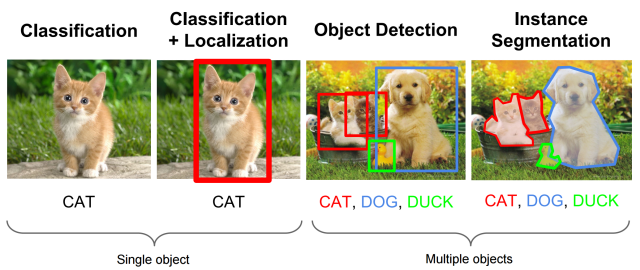
Levels in computer vision:
Level 1:- Image Classification (the network understands what is in an image)
Level 2:- Image Classification + Localization (Locates the object in the image)
Level 3:- Object Detection (Locates all objects in images)
Level 4:- Sematic Segmentation (Locates each object along with accurate shape/boundary of all objects)
Level 5:- Instance Segmentation (Locates multiple instances of same object)
(Level 1 and 2 are only for single object, rest can be used for multiple objects)
They used this in biomedical research, studying about different anatomy, diagnosing diseases etc...
But it was just inefficient. It required tens of thousands of training samples. Incase of biomedical, the success was limited due to the available size of training sets.
Until they invented U-Net, a convolutional neural network made for biomedical image segmentaion.
U-Net
U-Net was introduced to solve the inefficiency caused by existed computer vision in identifying biomedical images. U-Net was made completely using convolusional layers ⟶ that's how convolusions were made to help in computer vision. The whole point of convolusion is to extract features from an image.
Why was U-Net efficient?
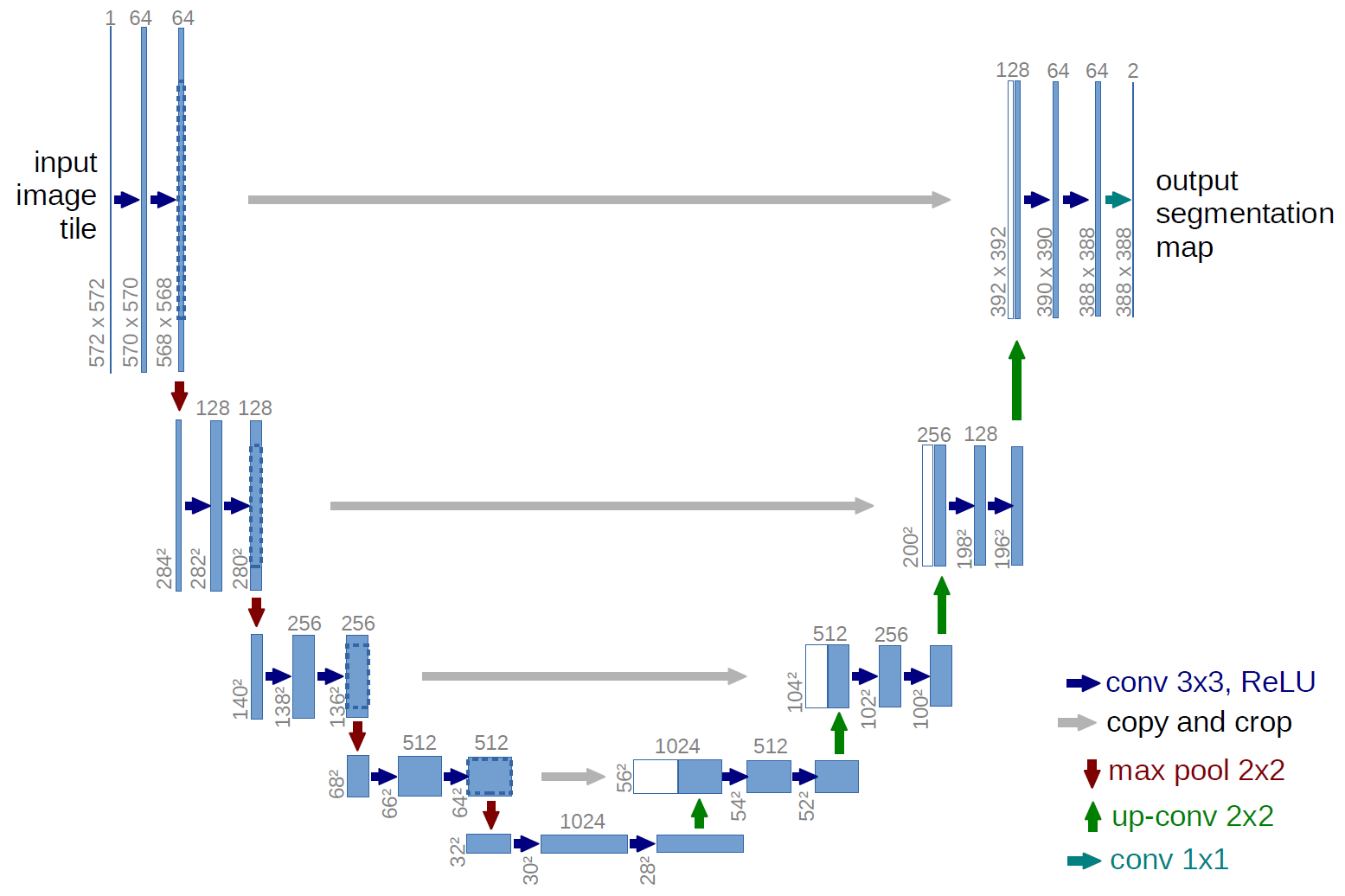
- U-Net can be divided into 2 parts(for understanding purpose) as left and right.
- U-Net has access over resolution of image(it can change resolution of the image) and number of channels(channel = features, kernels = feature extractors more kernels = more features can be indentified → more channels)
There is one issue with kernels identifying images, say you take a relatively large image like 256x256 and 5x5 kernel
- Kernel is too small to extract data from image
- To collect more data from image, kernel should be able to see more of an image.
How can this be solved? Either we can make kernels bigger like 7x7, 9x9 but this drastically increases number of parameters. This will make convolusions less efficient.
Another way is to make images smaller → Exactly what U-Net does
Hence in the left part of U-Net, it scales down the image, increases number of channels gradually so that it can identify all features of the image. Until it reaches maximum amount of channels and minimum res of image (halfway of U-Net and end of left part). Now it has all information about what is in the image but the downscaling of image has made it lose info on where it is in the image.
Hence in the right part of the U-Net, it starts to scale up the image and decrease the number of channels and finally merges everything to get actual segmented image.
The U-Net was so powerful that, just after training the U-Net with few 100s of images and segmented parts, it was able to work accurately.
It was so good at identifying such that people started to use it for other purposes. One of it was denoising.
U-net in denoising


For usual U-Net use aka for segmentation, in training we use images and segmented images.
Instead this time we feed noisy image and the noise, such that later on it can predict the noise, subtract it from noisy image and give us the actual image (rather than finding the segment, this time it will find the noise).
We feed the noisy image along with amount of noiseness in form of positional encoding. (Positional encoding is a type of embedding*, more positional encoding = more noise) This embedding vector gets drilled in the image in the network.
*embedding - converting disctere values like numbers/words to vectors which are digestible for neural network
Now after all this training, our network is good enough to denoise images. But, if we try to denoise, we still get unclear image. Why? It's because we try to denoise entirely in a single step (which is still too much for the network). Hence, we denoise completely, add 90% of the noise back, denoise again, add 90% of previous noise... The loop goes on until we get a clear image.
After all this training, the network will give us only one image, the image we trained it on.
So what if trained with 1000s of images of say a cat (noisy cat images and noise)? The network will now start generating completely new images of cats using the data we fed.
This is Diffusion Model
There are still some flaws in this method. For example, to generate HD images, it wkk take a lot of data and time to train on HD images. Reason? Since we are denoising pixel by pixel ie; directly on pixel → more pixels = more data = more time..
So is there a way to speed this up?
Latent Diffusion Model
To solve the above stated problem, people invented autoencoder.
Autoencoder is a neural network equivalent of encoding and decoding.
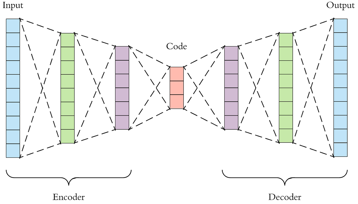
Here we will use autoencoder to encode the input images to it's compressed version in latent space. (This is similar to using jpeg which compresses and stored images instead of raw uncompressed pixel values) ie; The network can now use this low dimensional discriminative features rather than raw pixels (note: we are compressing the image representation, rather than compressing the image a losing out features, similar to tiff and jpeg)
noise image → (encode) → latent space → (denoise) → latent space → (decode) → output
This process is faster than denoising raw uncompressed data.
Word2Vec
So how does all of this help in generating images from texts? Using Word2Vec.
Word2Vec is a type of embedding(as we saw the definition of embedding previously)
It is a list of vectors, for each word used in the english language. There are two such lists, every word in the two lists have different vectors. (same word in both lists have different vectors)
Relation between vectors of words in same list:-
Words that are more likely to appear in similar contexts are grouped together (similar vectors)
Relation between vectors of words in different lists:-
Dot product of vectors of words(in different lists) is higher if the relationship between the two words is higher (more likely to appear together based on the data collected of texts ever written by humanity in books, internet etc...) Example: cute cat (vector[cute].vector[cat]) has higher dot product than cute table (vector[cute].vector[cat]), since cute cat appears more together than cute table.
These vectors are so accurate that you can add/subtract them to get new/similar words. Example: Vec(King) - Vec(Man) + Vec(Woman) = Vec(Queen)

Attention Layer
Convolution: Extract features from images using relation between pixels and their relative spatial position
Self Attention(the attention layer we use here): Extract features from images using relation between words depending on embedding vectors
Self Attention Layer is similar to fully connected layer (basic layer which we saw in introduction section) but
- Each input and output are vectors
- Weights of /values on connection is the dot product of the connecting vectors
Let's take two pairs of words say "not good" and "good not", obviously "not good" makes more sense than "good not" but if you take dot product of both sets of words, you will get same value.
To solve this issue, we take 3 variables
- Query
- Key
- Value
Take Vec(A).Vec(B) where A and B are two words, query is related to B(second word), key is related to A(first word) and value is related to the output produced by A and B. Instead of taking Query, key and value as variables, we take it as vectors instead. After multiplying these vectors to A and B respectively, we will get different values for Vec(A).Vec(B) and Vec(B).Vec(A) ie; different values for "not good" and "good not".
For more than two words, we can use CBOW/Continuous Skip-Gram model to extract the relation between the words and finally convert them to vectors so that our network can understand.
Using conolutional layer, we can encode an image into embedding vector. Using attention layer, we can encode a text to embedding vector, what if both layers display same vectors?
That is what openAI tried to do, training on 400 million images, so images and text that match, will come up with same vectors.
Since here we are using two kinds of inputs, image and text, instead of self attention layer, we use cross attention layer(operates on two sets of data, image and text). Therefore it works by modifying input image with guide of text input, creating new creative output image. This is how we eventually train the network to generate image based on text input.
Conclusion
Convolusional layer learns images
Attention layer learns texts
When you combine the two, you generate images based on text.
(Definitely took a lot of time to make this blog)


Comments
Post a Comment